Linear Regression From Scratch

Linear regression is one of the fundamental algorithms in supervised machine learning. Its simplicity makes it an excellent starting point for understanding how models learn relationships from data, measure prediction errors, and optimize their parameters.

This article explains the mathematical intuition behind linear regression and its implementation from scratch. The discussion covers the Normal Equation, gradient descent, polynomial regression, regularization techniques, and model-complexity control.

The Hypothesis Function

Linear regression models the relationship between input features and a continuous target variable, such as predicting house prices based on size, bedrooms, and age.

The model assumes that the target can be approximated by a linear combination of the input features. The weights and bias are learned from historical data to minimize prediction error. Predictions are generated by the hypothesis function, which mathematically represents the line, plane, or hyperplane fitted to the data.

For simple linear regression, which uses one feature:

$$\hat{y} = wx + b$$

For multiple linear regression, which uses several features:

$$\hat{y} = w_1x_1 + w_2x_2 + \cdots + w_px_p + b$$

Here, \(\hat{y}\) is the predicted value, $x$ represents an input feature, $w$ is its weight or coefficient, and $b$ is the bias or intercept. The weight determines how the prediction changes with the corresponding feature, while the bias shifts the prediction independently of the feature values.

The objective is to find the weights and bias that produce predictions as close as possible to the actual target values.

Example Data: House Prices vs. Square Footage

Consider the following dataset of house prices based on square footage:

# X layout: [Square Footage]

X = np.array([1000, 1100, 1200, 1300, 1400, 1500, 1600, 1700, 1800, 2000], dtype=float)
X = X.reshape(-1,1)
# y layout: [House Price]
y = np.array([150000, 165000, 180000, 210000, 220000, 240000, 265000, 270000, 285000, 320000], dtype=float)
print(f"Number of training examples (m): {X.shape[0]}")
print(f"Number of features (n): {X.shape[1]}")
# Number of training examples (m): 10
# Number of features (n): 1

There are 10 data points (\(m = 10\)), and 1 feature (\(n = 1\)).

The Cost Function

A cost function measures how far the model's predictions are from the actual values. It provides a numerical objective that can be minimized to find suitable model parameters.

Mean Squared Error (MSE):

Mean Squared Error is a widely used cost function for linear regression. It calculates the average of the squared differences between actual and predicted values.

$$J(w,b) = \frac{1}{m}\sum_{i=1}^{m}(y_i-\hat{y}_i)^2$$

Where:

- $m$ is the number of training examples.

- \(y_i\) is the actual value for example $i$.

- \(\hat{y}_i\) is the predicted value for example $i$.

Squaring the errors prevents positive and negative errors from cancelling each other out and penalizes larger errors more heavily. MSE is also differentiable, making it convenient for gradient descent. However, it is sensitive to outliers because large errors contribute disproportionately to the cost.

Implementation of MSE:

def mean_squared_error(y_true, y_pred):
    errors = y_true - y_pred
    return np.mean(errors ** 2)

Other cost functions include Mean Absolute Error (MAE) which is less sensitive to outliers than MSE and Huber Loss which combines the strengths of both.

The Normal Equation

The Normal Equation provides a closed-form solution to find the parameters that minimize the cost function without requiring iterative updates like Gradient Descent. It calculates the optimal weights and bias that achieve the lowest possible error in a single analytical step.

Expressing Linear Regression in Matrix Form

To compute predictions for all $m$ training examples simultaneously, linear regression can be expressed as a vectorized matrix formulation. the bias term is absorbed (\(b = w_0\)) into the parameter vector \(\mathbf{W}\) alongside a corresponding dummy feature (\(x_0 = 1\)) inside the design matrix \(\mathbf{X}\):

$$\hat{\mathbf{y}} = \mathbf{X}\mathbf{W}$$

Written out explicitly, the matrix dimensions align as:

$$\begin{bmatrix} \hat{y}^{(1)} \ \hat{y}^{(2)} \ \vdots \ \hat{y}^{(m)} \end{bmatrix} = \begin{bmatrix} 1 & x_{1}^{(1)} & \dots & x_{n}^{(1)} \ 1 & x_{1}^{(2)} & \dots & x_{n}^{(2)} \ \vdots & \vdots & \ddots & \vdots \ 1 & x_{1}^{(m)} & \dots & x_{n}^{(m)} \end{bmatrix} \begin{bmatrix} b \ w_{1} \ \vdots \ w_{n} \end{bmatrix}$$

Where:

• \(\hat{\mathbf{y}}\) is the \((m \times 1)\) vector of predicted target values.
• \(\mathbf{W}\) is the \(((n+1) \times 1)\) parameter vector containing the bias and weights.
• \(\mathbf{X}\) is the \((m \times (n+1))\) design matrix containing all feature inputs.

The Cost Function and Vectorized Gradient

The Mean Squared Error (MSE) cost function can be expressed in compact matrix form:

$$J(\mathbf{W}) = \frac{1}{m} (\mathbf{X}\mathbf{W} - \mathbf{y})^T (\mathbf{X}\mathbf{W} - \mathbf{y})$$

Computing the matrix of partial derivatives with respect to the parameters yields the gradient vector \(\frac{\partial J}{\partial \mathbf{W}}\):

$$\frac{\partial J}{\partial \mathbf{W}} = \frac{2}{m}\mathbf{X}^T\left(\mathbf{X}\mathbf{W} - \mathbf{y}\right)$$

The Closed-Form Solution

Setting the gradient vector to zero (\(\frac{\partial J}{\partial \mathbf{W}} = \mathbf{0}\)) identifies the minimum of the cost function. Solving this matrix equation yields the Normal Equation:

$$\boxed{ \mathbf{W} = (\mathbf{X}^T \mathbf{X})^{-1}\mathbf{X}^T\mathbf{y} }$$

X = np.asarray(X, dtype=float)
y = np.asarray(y, dtype=float).reshape(-1)
# add a column of ones to the left side of the feature matrix X

X_new = np.column_stack([np.ones(X.shape[0]),X])
W = np.dot(np.linalg.inv(np.dot(X_new\.T, X_new)), np.dot(X_new\.T, y))
y_pred = np.dot(X_new, coefficients)
mse = mean_squared_error(y, y_pred)
print(f"Bias: {W[0]} | Weight: {W[1]}")
print(f"Mean Square Error: {mse}")

# Result:
# Bias: -21049.78354978488 | Weight: 172.2943722943726
# Mean Square Error: 24323593.07359312

This approach avoids tuning a learning rate (\(\alpha\)) or tracking convergence loops. However, computing the raw matrix inverse \((\mathbf{X}^T \mathbf{X})^{-1}\) requires roughly \(\mathcal{O}(n^3)\) computational time, meaning it scales poorly as the number of features ($n$) grows.

Instead of computing that matrix inverse directly, np.linalg.lstsq uses a highly optimized technique called Singular Value Decomposition (SVD). It computes the "pseudo-inverse" of the features to return the weights that minimize the Mean Squared Error function, avoiding runtime crashes caused by redundant or highly correlated features.

coefficients, residuals, _, _ = (np.linalg.lstsq(X_new, y, rcond=None))
print(f"Bias: {coefficients[0]} | Weight: {coefficients[1]}")
print(f"Mean Square Error: {residuals[0]}")
y_pred = np.dot(X_new, coefficients)

# Result:
# Bias: -21049.783549783482 | Weight: 172.29437229437232
# Mean Square Error: 243235930.73593095

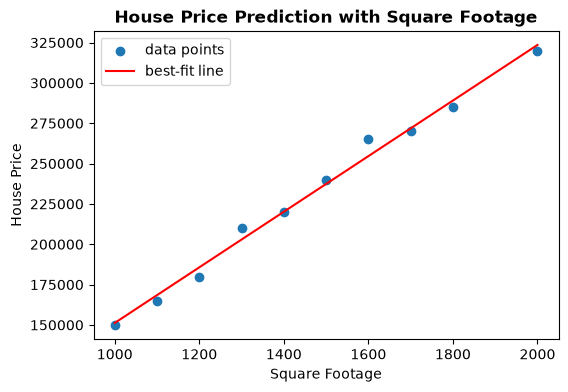
the model can visualize the predicted house prices:

plt.figure(figsize=(6, 4))
plt.scatter(X, y, c='blue', marker='x')
plt.plot(X, y_pred, c='red', label='Best-fit line')
plt.title("House Prices vs. Square Footage")
plt.xlabel("Square Footage (x)")
plt.ylabel("Price in Dollars (y)")
plt.grid(True)
plt.show()

Gradient Descent

Gradient descent finds optimal model parameters by iteratively moving in the direction that reduces the cost function. The general update rule is:

$$\mathbf{W}_{\text{next}} = \mathbf{W} - \alpha \frac{\partial J}{\partial \mathbf{W}}$$

Where \(\alpha\) represents the learning rate, controlling the step size taken down the error surface.

The Cost Function and Matrix Gradient

To find the gradient vector \(\frac{\partial J}{\partial \mathbf{W}}\), the model define the objective using the matrix form of the Mean Squared Error (MSE):

$$J(\mathbf{W}) = \frac{1}{m} (\mathbf{X}\mathbf{W} - \mathbf{y})^T (\mathbf{X}\mathbf{W} - \mathbf{y})$$

Computing the partial derivatives of this cost function with respect to the model parameters yields the global gradient vector:

$$\frac{\partial J}{\partial \mathbf{W}} = \frac{2}{m}\mathbf{X}^T(\mathbf{X}\mathbf{W} - \mathbf{y})$$

Batch Gradient Descent

Batch Gradient Descent evaluates the gradient across the entire training dataset ($m$ samples) to make a single parameter update. Substituting the matrix gradient into the general update rule gives:

$$\boxed{ \mathbf{W}_{\text{next}} = \mathbf{W} - \alpha \frac{2}{m}\mathbf{X}^T(\mathbf{X}\mathbf{W} - \mathbf{y}) }$$

While this approach creates a smooth, direct trajectory toward the global minimum, processing the full design matrix \(\mathbf{X}\) becomes computationally heavy on massive datasets.

Implementation of batch gradient descent with a learning rate of 0.01 and 1000 iterations:

def batch_gradient_descent(X, y, learning_rate=0.01, n_iterations=1000):
    X = np.asarray(X, dtype=float)
    y = np.asarray(y, dtype=float).reshape(-1)
    n_samples, n_features = X.shape
    # Create the Design Matrix by adding the intercept column (x0 = 1)

    X_new = np.column_stack([np.ones(n_samples), X])
    # Initialize unified parameter vector W: [bias, w1, w2, ..., wn] to zeros

    W = np.zeros(n_features + 1)
    loss_history = []

    for _ in range(n_iterations):
        # compute y_pred based on y_pred = X.W
        y_pred = np.dot(X_new, W)
        error = y_pred - y
        # Calculate and store loss
        mse = np.mean(error ** 2)
        loss_history.append(mse)
        # calculate and update new parameters
        dw = (2 / n_samples) * np.dot(X_new\.T, error)
        W -= learning_rate * dw

    bias = W[0]
    weights = W[1:]
    return bias, weights, loss_history

Stochastic Gradient Descent (SGD)

Stochastic Gradient Descent drops the global matrix operation entirely, updating parameters sequentially using only one randomly selected training instance \(\mathbf{x}^{(i)}\) and target \(y^{(i)}\) at a time (\(m=1\)). For an individual sample $i$, the update rule simplifies to:

$$\mathbf{W}_{\text{next}} = \mathbf{W} - 2\alpha \mathbf{x}^{(i)T}(\mathbf{x}^{(i)}\mathbf{W} - y^{(i)})$$

SGD drastically reduces computational overhead per iteration, though single-sample noise causes the cost function to fluctuate during training. Incorporating a learning rate schedule that decays \(\alpha\) over time helps the parameters stabilize near the global minimum.

The Stochastic Gradient Descent implementation is as follows:

def stochastic_gradient_descent(X, y, learning_rate=0.01, n_epochs=50):
    X = np.asarray(X, dtype=float)
    y = np.asarray(y, dtype=float).reshape(-1)
    n_samples, n_features = X.shape
    X_new = np.column_stack([np.ones(n_samples), X])
    W = np.zeros(n_features + 1)
    loss_history = []
    for epoch in range(n_epochs):
        indices = np.random.permutation(n_samples)
        for i in indices:
            Xi = X_new[i]
            yi = y[i]
            yi_pred = np.dot(Xi, W)
            error = yi_pred - yi
            dw = 2 * error * Xi
            W -= learning_rate * dw
        epoch_y_pred = np.dot(X_new, W)
        epoch_error = epoch_y_pred - y
        epoch_loss = np.mean(epoch_error ** 2)
        loss_history.append(epoch_loss)
    bias = W[0]
    weights = W[1:]
    return bias, weights, loss_history

Mini-Batch Gradient Descent

Mini-Batch Gradient Descent strikes a practical middle ground, calculating the gradient over a fixed subset of the data containing $k$ examples. For a mini-batch slice \(\mathbf{X}_B\) and its corresponding target array \(\mathbf{y}_B\):

$$\mathbf{W}_{\text{next}} = \mathbf{W} - \alpha \frac{2}{k}\mathbf{X}_B^T(\mathbf{X}_B\mathbf{W} - \mathbf{y}_B)$$

This variant balances the speed of SGD with the trajectory stability of Batch Gradient Descent, maximizing performance by mapping efficiently onto vectorized hardware array operations.

The following code implements mini-batch gradient descent:

def mini_batch_gradient_descent(X, y, learning_rate=0.01, n_epochs=50, batch_size=50):
    X = np.asarray(X, dtype=float)
    y = np.asarray(y, dtype=float).reshape(-1)
    n_samples, n_features = X.shape
    X_new = np.column_stack([np.ones(n_samples), X])
    W = np.zeros(n_features + 1)
    loss_history = []
    for epoch in range(n_epochs):
        indices = np.random.permutation(n_samples)
        X_shuffled = X_new[indices]
        y_shuffled = y[indices]
        for i in range(0, n_samples, batch_size):
            X_batch = X_shuffled[i : i + batch_size]
            y_batch = y_shuffled[i : i + batch_size]
            k, _ = X_batch.shape
            y_batch_pred = np.dot(X_batch, W)
            batch_error = y_batch_pred - y_batch
            dw = (2 / k) * np.dot(X_batch.T, batch_error)
            W -= learning_rate * dw
        epoch_y_pred = np.dot(X_new, W)
        epoch_error = epoch_y_pred - y
        epoch_loss = np.mean(epoch_error ** 2)
        loss_history.append(epoch_loss)
    bias = W[0]
    weights = W[1:]
    return bias, weights, loss_history

Polynomial Regression

Polynomial regression enables linear models to capture complex, curved relationships by projecting the original input features into a higher-dimensional space using feature transformations (e.g., \(x^2, x^3, \dots, x^n\)).

$$\hat{y} = b + w_1x + w_2x^2 + \cdots + w_nx^n$$

Although the relationship between the prediction \(\hat{y}\) and the raw input $x$ is highly nonlinear, the model remains fundamentally linear with respect to its parameters \(\mathbf{W}\). Consequently, the exact same vectorized optimization routines, such as Gradient Descent and the Normal Equation, can be applied directly after the feature matrix has been transformed via a basis mapping function \(\phi(x)\).

Using an excessively high polynomial degree $n$ can lead to overfitting, where the model captures the noise within the training matrix instead of the underlying distribution, resulting in poor generalization on unseen data.

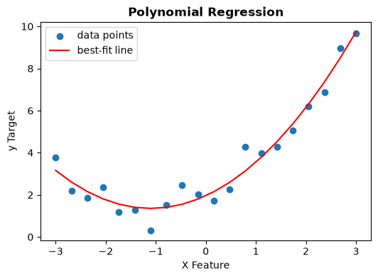
Consider the following sample dataset with a quadratic relationship between the input and output variables. Polynomial regression model works by stacking powers to the input feature matrix.

X = np.linspace(-3, 3, 20).reshape(-1, 1)
noise = np.random.normal(0, 0.5, size=(20, 1))
y = (0.5 * (X ** 2) + 1.0 * X + 2.0 + noise).reshape(-1)
# Stacking a column of X^2 to X to create a polynomial feature matrix
X_poly = np.column_stack([X, X ** 2])
bias, weights, loss_history = batch_gradient_descent(
X_poly, y, learning_rate=0.01, n_iterations=1000)

y_pred = X_poly @ weights + bias
plt.figure(figsize=(6,4))
plt.scatter(X,y, label="data points")
plt.plot(X,y_pred, color="r", label="best-fit line")
plt.title("Polynomial Regression", fontweight="bold")
plt.xlabel("X Feature")
plt.ylabel("y Target")
plt.legend()
plt.show()

Regularization

Regularization introduces a structural penalty to the cost function to discourage excessively large parameter values. By constraining the magnitude of the feature weights, it controls model complexity and reduces overfitting.

Note: In alignment with machine learning conventions, the bias term $b$ (or \(w_0\)) is conventionally excluded from the regularization penalty to avoid forcing the model's intercept baseline toward zero.

Ridge Regression (\(L_2\) Regularization)

Ridge regression adds a penalty proportional to the sum of the squared feature weights to the Mean Squared Error (MSE) cost function.

$$J(\mathbf{W}) = \frac{1}{m} (\mathbf{X}\mathbf{W} - \mathbf{y})^T (\mathbf{X}\mathbf{W} - \mathbf{y}) + \frac{\lambda}{m}\sum_{j=1}^{n}w_j^2$$

The regularization parameter \(\lambda\) controls the penalty strength. Increasing \(\lambda\) shrinks the weights asymptotically toward zero, reducing model variance, though it generally does not zero them out completely.

Lasso Regression (\(L_1\) Regularization)

Lasso (Least Absolute Shrinkage and Selection Operator) regression adds a penalty proportional to the sum of the absolute values of the feature weights.

$$J(\mathbf{W}) = \frac{1}{m} (\mathbf{X}\mathbf{W} - \mathbf{y})^T (\mathbf{X}\mathbf{W} - \mathbf{y}) + \frac{\lambda}{m}\sum_{j=1}^{n}|w_j|$$

Because of the geometry of the \(L_1\) diamond-shaped constraint space, Lasso acts as an automated feature selection tool by driving non-essential feature weights precisely to zero (\(w_j = 0\)).

Elastic Net

Elastic Net provides a hybrid approach by combining both the \(L_1\) and \(L_2\) regularization penalties into a single cost function.

$$J(\mathbf{W}) = \frac{1}{m} (\mathbf{X}\mathbf{W} - \mathbf{y})^T (\mathbf{X}\mathbf{W} - \mathbf{y}) + \frac{\lambda r}{m}\sum_{j=1}^{n}|w_j| + \frac{\lambda(1-r)}{m}\sum_{j=1}^{n}w_j^2$$

In this formulation, \(\lambda\) controls the overall regularization intensity, while the mixing ratio $r$ balances the structural properties of both frameworks. Setting \(r=1\) yields pure Lasso regression, while setting \(r=0\) reduces the expression back to Ridge regression.

Evaluating model performance with R² Score

The raw numerical value of Mean Squared Error (often in the millions or billions) can be difficult to interpret directly. The R² Score (Coefficient of Determination) provides another measure of how well the model fits the data.

The R² score represents the proportion of variance in the target variable (y) that can be predicted from the input features (X). It essentially compares the model's predictions against a baseline model that simply guesses the average target value (ȳ) for every single house.

Mathematical Formulation

The R² score is defined as:

$$R^2 = 1 - \frac{SS_{\text{res}}}{SS_{\text{tot}}}$$

Where:

• (Residual Sum of Squares): The sum of squared errors between the model predictions and the true values. This is directly related to the MSE.

$$SS_{\text{res}} = \sum_{i=1}^{m} \left(y^{(i)} - \hat{y}^{(i)}\right)^2$$

• (Total Sum of Squares): The total variance present in the true data points relative to their baseline mean (ȳ).

$$SS_{\text{tot}} = \sum_{i=1}^{m} \left(y^{(i)} - \bar{y}\right)^2$$

R² = 1.0 (100%) shows a Perfect model, R² = 0.0 (0%) shows a model that performs no better than simply guessing the average house price every time and R² < 0.0 shows a model that performs worse than guessing the average value. This typically indicates a major mathematical implementation bug or an unscaled model explosion.

Vectorized Python Implementation of the R² score

def r2_score(y_true, y_pred, epsilon=1e-15):
    y_true = np.asarray(y_true, dtype=float).reshape(-1)
    y_pred = np.asarray(y_pred, dtype=float).reshape(-1)
    y_mean = np.mean(y_true)
    ss_res = np.sum((y_true - y_pred) ** 2)
    ss_tot = np.sum((y_true - y_mean) ** 2)
    r2 = 1.0 - (ss_res / (ss_tot + epsilon))
    return r2

# Generate predictions using the trained scaled parameters

y_pred_none = X_scaled @ w_none + b_none
y_pred_ridge = X_scaled @ w_ridge + b_ridge
# Compute performance ratios
print(f"R² Score (No Penalty):  {r2_score(y, y_pred_none) * 100:.2f}%")
print(f"R² Score (Ridge Penalty): {r2_score(y, y_pred_ridge) * 100:.2f}%")

# Result:
# R² Score (No Penalty):  62.29%
# R² Score (Ridge Penalty): 60.47%

**The link below contains the full implementation. **

Linear regression from scratch full implementation