Logistic Regression in Python: Math to Implementation

Logistic regression is a supervised machine learning algorithm used for classification tasks, particularly binary classification, where the goal is to predict one of two possible classes. Unlike linear regression, which predicts continuous numerical values, logistic regression estimates the probability that an observation belongs to a particular class. It achieves this by applying an activation function, called the sigmoid function, to a linear combination of the input features and their corresponding weights and bias. The sigmoid function transforms the model's output into a probability score between 0 and 1, which can then be used to determine the predicted class based on a classification threshold.

Given an input feature vector X, a logistic regression model outputs a prediction representing the probability that the target variable belongs to the positive class (class 1), conditioned on the input features X:

$$\hat{y} = P(y=1 \mid x)$$

Since this is a probability:

$$0 \leq \hat{y} \leq 1$$

Sigmoid Function

The sigmoid function, also known as the logistic function, is an activation function that maps any real-valued input into a range between 0 and 1. In logistic regression, it is used to transform the output of a linear equation into a probability.

In linear regression, the hypothesis function is expressed as:

$$\hat{y} = wX + b$$

Where:

• x represents the input feature vector.
• w represents the weight vector assigned to the input features.
• b represents the bias (intercept).

However, the output of this linear equation can take any real value, ranging from negative infinity to positive infinity. This makes it unsuitable for directly representing a probability, which must fall strictly between 0 and 1.

To address this, logistic regression passes the output of the linear equation through the sigmoid function.

The sigmoid function is defined as:

$$\boxed{ \sigma(z) = \frac{1}{1+e^{-z}} }$$

Where:

• z is the input to the sigmoid function.
• e is Euler's number (approximately 2.71828).
• Sigma of z represents the output of the sigmoid function.

In logistic regression, z is the linear combination of the input features, weights, and bias:

$$z = wX + b$$

For multiple input features:

$$z = w_1x_1 + w_2x_2 + \cdots + w_px_p + b$$

Substituting this linear combination into the sigmoid function yields the logistic regression hypothesis function:

$$\boxed{\hat{y} = \sigma(wX+b)}$$

Or, written out with individual features:

$$\boxed{ \hat{y} = \frac{1}{1+e^{-(w_1x_1+w_2x_2+\cdots+w_px_p+b)}} }$$

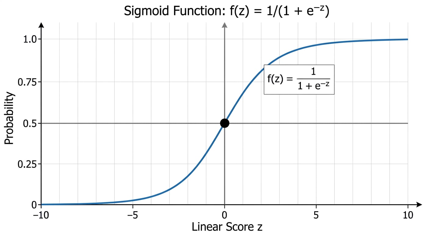
The sigmoid function has an S-shaped curve as shown below. Regardless of how large or small the input is, the output always falls between 0 and 1.

Important properties of the sigmoid function:

1. When z equals 0, the output is exactly 0.5.
2. For positive values of z, the output is greater than 0.5, asymptotically approaching 1.
3. For negative values of z, the output is less than 0.5, asymptotically approaching 0.
4. The output is strictly bounded between 0 and 1, making it well-suited for probability estimation.

The sigmoid function produces a continuous probability, but classification requires assigning an observation to a specific discrete class label (0 or 1). This is achieved by setting a classification threshold. The standard default threshold in binary logistic regression is 0.5:

$$y_{\text{pred}} = \begin{cases} 1, & \text{if } \hat{y} \geq 0.5\\ 0, & \text{if } \hat{y} < 0.5 \end{cases}$$

However, the 0.5 threshold is a default rather than a fixed constraint. The threshold can be adjusted depending on the specific application and the relative costs associated with false positives versus false negatives.

While the sigmoid function enables logistic regression to convert a linear output into a probability, a method is required to measure how close these predicted probabilities are to the actual class labels. This role is fulfilled by the cost function.

Implementation with NumPy:

def sigmoid(z):
    """Compute the sigmoid of z."""
    y_hat = 1 / (1 + np.exp(-z))
    return y_hat

Cost Function

The cost function measures how well a machine learning model's predictions align with the actual target values. It quantifies the error between the predicted values and the actual values, providing an objective value that the learning algorithm minimizes during training.

Although Mean Squared Error (MSE) can mathematically measure the difference between predicted probabilities and actual binary labels, it is not the preferred cost function for logistic regression. When combined with the sigmoid function, MSE produces a non-convex cost surface with multiple local minima and saddle points, making gradient-based optimization difficult. Instead, logistic regression uses Binary Cross-Entropy (BCE), also known as Log Loss, as the cost function.

Binary Cross-Entropy (Log Loss)

Binary Cross-Entropy (BCE) measures the difference between actual binary labels and the probabilities predicted by the model. It heavily penalizes confident predictions that turn out to be incorrect. For a single training example, the Binary Cross-Entropy loss function is defined as:

$$L(\hat{y},y) = -\left[y\log(\hat{y})+(1-y)\log(1-\hat{y})\right]$$

Where:

• y is the actual binary label (0 or 1).
• y-hat is the predicted probability that the observation belongs to class 1.
• log denotes the natural logarithm.

The objective of Binary Cross-Entropy is to penalize deviations between the predicted probability and the true class label:

• When the actual label is 1, the second term drops out, leaving the negative logarithm of the predicted probability. Minimizing this loss pushes the predicted probability toward 1.

• Conversely, when the actual label is 0, the first term drops out, leaving the negative logarithm of one minus the predicted probability. Minimizing this loss pushes the predicted probability toward 0.

In this manner, the loss function steers the model toward outputting high probabilities for the true class and low probabilities for the incorrect class.

Cost Function for the Entire Training Dataset

The loss function calculates the error for an individual training example. To measure overall performance across the entire training dataset, the average loss across all m training examples is calculated.

The Binary Cross-Entropy cost function is defined as:

$$\boxed{ J(w,b) = -\frac{1}{m}\sum_{i=1}^{m} \left[ y^{(i)}\log(\hat{y}^{(i)}) + (1-y^{(i)})\log(1-\hat{y}^{(i)}) \right] }$$

Where:

• m is the total number of training examples.
• y for the i-th training example is the actual label.
• y-hat for the i-th training example is the predicted probability.

The predicted probability is obtained from the hypothesis function:

$$\hat{y}^{(i)} = \sigma(w^Tx^{(i)}+b)$$

Substituting this hypothesis into the cost function yields the complete objective that logistic regression minimizes:

$$J(w,b) = -\frac{1}{m}\sum_{i=1}^{m} \left[ y^{(i)}\log(\sigma(w^Tx^{(i)}+b)) + (1-y^{(i)})\log(1-\sigma(w^Tx^{(i)}+b)) \right]$$

The next step is to minimize this Binary Cross-Entropy cost function by finding the optimal weights and bias. This optimization is performed using gradient descent.

Binary Cross-Entropy implementation with NumPy:

def cost_function(y, y_hat):
    """Compute the Binary Cross-Entropy cost across m examples."""
    m = y.shape[0]
    epsilon = 1e-9  # Prevents numerical instability (log(0))
    cost = - (1 / m) * np.sum(y * np.log(y_hat + epsilon) + (1 - y) * np.log(1 - y_hat + epsilon))
    return cost

Gradient Descent

Gradient descent is an optimization algorithm used to minimize the cost function by iteratively adjusting the model parameters (weights and bias) in the direction of steepest descent.

In logistic regression, gradient descent is applied to find the optimal weights and bias that minimize the Binary Cross-Entropy cost function. The algorithm computes the partial derivatives (gradients) of the cost function with respect to each parameter and uses them to iteratively update those parameters.

To apply gradient descent, the partial derivatives of the cost function with respect to the weights and bias must be computed. The partial derivatives of the loss function with respect to the weight vector w and bias b for a single training example are:

$$\begin{aligned} \frac{\partial L}{\partial w} &= (\hat{y}-y)x &\qquad \frac{\partial L}{\partial b} &= \hat{y}-y \end{aligned}$$

This expression yields the gradient of the loss function with respect to the parameters for a single observation. Because the cost function computes the average loss across all m training examples, the gradients of the overall cost function are obtained by taking the average across all examples:

$$\begin{aligned} \frac{\partial J}{\partial w} &= \frac{1}{m}\sum_{i=1}^{m} (\hat{y}^{(i)}-y^{(i)})x^{(i)} \[8pt] \frac{\partial J}{\partial b} &= \frac{1}{m}\sum_{i=1}^{m} (\hat{y}^{(i)}-y^{(i)}) \end{aligned}$$

The vectorized notation for the weight and bias gradients across all m training examples is:

$$\boxed{ \begin{aligned} \frac{\partial J}{\partial w} &= \frac{1}{m}X^T(\hat{Y}-Y) &\qquad \frac{\partial J}{\partial b} = \frac{1}{m}\mathbf{1}^T(\hat{Y}-Y) \end{aligned} }$$

Here, the matrix multiplication X-transpose multiplied by the prediction errors computes the gradient for each weight simultaneously, with every feature contributing its corresponding value to the gradient vector. For the bias, the prediction errors are summed across all training examples because the bias is a single parameter shared across every observation. Where:

• X is the input feature matrix with shape (m, n).
• Y-hat is the vector of predicted probabilities with shape (m, 1).
• Y is the vector of actual labels with shape (m, 1).
• m is the number of training examples.
• X-transpose is the transpose of the feature matrix with shape (n, m).

Gradient descent is an iterative procedure that updates the parameters in the direction opposite to their gradients. The update rules for the weights and bias are:

$$\begin{aligned} w &:= w-\alpha\frac{\partial J}{\partial w} &\qquad b &:= b-\alpha\frac{\partial J}{\partial b} \end{aligned}$$

The learning rate, alpha, determines the step size for each iteration. A learning rate that is too large can cause the algorithm to overshoot the minimum, whereas a learning rate that is too small slows down convergence.

Both gradients are governed by the difference between the predicted probability and the actual label. This quantity represents the prediction error or residual.

In the model implementation, the forward propagation and backward gradient computation are combined in the _propagate method:

def _propagate(self, X, y):
    # Forward propagation (from X to cost)
    m, n = X.shape
    z = np.dot(X, self.weights) + self.bias
    y_hat = self._sigmoid(z)
    cost = self._cost_function(y, y_hat)

    # Backward propagation (to find gradients)
    error = y_hat - y
    dw = (1 / m) * np.dot(X.T, error)
    db = (1 / m) * np.sum(error)
    return dw, db, cost

Once the model has learned the optimal weights and bias during training, it is deployed to make predictions on unseen data.

The first step computes the predicted probability by taking the linear combination of the input features and applying the sigmoid function:

$$\boxed{\hat{y} = \sigma(Xw+b)}$$

For binary classification, y-hat represents the probability that an observation belongs to class 1. The probability of belonging to class 0 is therefore one minus that probability.

This is implemented in the predict_proba() method, which outputs the probabilities for both classes:

def predict_proba(self, X):
    z = np.dot(X, self.weights) + self.bias
    y_prob_1 = self._sigmoid(z).ravel()
    y_prob_0 = 1 - y_prob_1
    return np.column_stack((y_prob_0, y_prob_1))

The returned array contains two columns: the first contains the probabilities for class 0, and the second contains the probabilities for class 1.

To obtain the final discrete class predictions, a classification threshold is applied. By default, a threshold of 0.5 is used: observations with a predicted probability of 0.5 or higher are assigned to class 1; otherwise, they are assigned to class 0.

def predict(self, X):
    y_prob = self.predict_proba(X)[:, 1]
    y_pred = (y_prob >= 0.5).astype(int)
    return y_pred

Here, [:, 1] selects the probability of class 1 from the second column of predict_proba(). The threshold comparison then converts these continuous probabilities into discrete binary class labels.

Conclusion

The sigmoid function transforms the linear output of logistic regression into a valid probability between 0 and 1. This probability is then compared against a classification threshold to determine the final predicted class.

Binary Cross-Entropy measures the discrepancy between actual binary labels and the probabilities predicted by the model. During training, the model iteratively adjusts its weights and bias via gradient descent to minimize this cost function, improving its capability to distinguish between the two classes.

Full implementation link

Logistic Regression from Scratch Python Implementation